2023-04-24：论文速递

1、Reference-based Image Composition with Sketch via Structure-aware Diffusion Model

结合手绘草图和参考图像提供的信息，通过一个结构感知的扩散模型，实现对目标图像结构的控制和修改。

《Reference-based Image Composition with Sketch via Structure-aware Diffusion Model》

• URL：https://arxiv.org/abs/2304.09748

• Official Code：Paint-by-Sketch

• 单位：韩国科学技术院（KAIST）

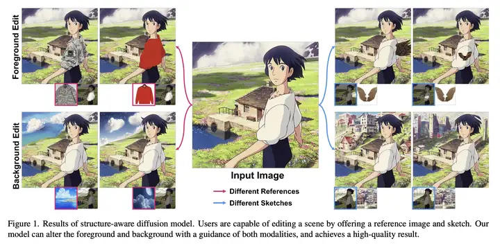
• 动机：通过利用 手绘草图（Sketch） 和 参考图像（Reference-based Image） 的局部信息，实现用户 对目标图像结构的控制和修改（Image Paint）。

• 方法：使用 多输入条件 的图像合成模型，以手绘草图和参考图像为输入，在生成过程中 草图提供结构引导，参考图像提供语义信息，微调 预训练扩散模型，填充缺失区域（Mask / Missing Region）。

• 优势：用户能使用所需结构的草图和内容的参考图像编辑或完整图像的某个子部分，具有较高的灵活性和可控性，同时能够 适应多种不同的草图类型。

1.1、问题描述

现有的 text-to-image diffusion model 的训练过程如下：

an encoder \(\varepsilon\) encodes \(\mathbf{x}\) into a latent representation \(z = \varepsilon(\mathbf{x})\), and a decoder \(D\) reconstructs the image from \(z\).

a conditional diffusion model \(\epsilon_θ\) is trained with the following loss function:

其中，

• \(\mathbf{x} \in R^{3\times H\times W}\) 表示 input image

  • 其中，\(H\) 和 \(W\) 分别代表 input image 的宽高

• \(\mathbf{y}\) 表示 text condition，并且送入到 预训练的 CLIP text encoder，即 \(\text{CLIP}(\mathbf{y})\)

• \(t\) is uniformly sampled from \(\{1, ..., T\}\)

• \(z_t\) is a noisy version of the latent representation \(z\)

• 潜在扩散模型使用 时间条件（time-conditioned）的 U-Net 作为 \(\epsilon_θ\)

To achieve the faster convergence of our method, we employ Stable Diffusion as a strong prior. 也就是说，作者 对 Stable Diffusion 进行了微调，而非从头开始训练一个 Diffusion Model。

具体的这篇文章，

• \(\mathbf{x}_p \in R^{3\times H\times W}\) 表示原始图像

• \(m\in \{0, 1\}^{H\times W}\) 表示一个二值 (binary) Mask

• \(s\in \{0, 1\}^{H\times W}\) 表示 Sketch Image

  • 提供 Mask Region 的 结构信息

• \(\mathbf{x}_r\in R^{3\times H'\times W'}\) 表示 Reference Image

  • 提供 Sketch 内部所需的 语义信息

1.2、具体方法

1）训练阶段

在训练期间，模型使用 参考图像的内容 填充 遵循草图引导结构 的蒙版区域。

We take self-supervised training to train a diffusion model，具体的前向过程如下所示。

对于每个训练迭代过程：

• 每个 batch 由 \(\{\mathbf{x}_p, m, s, \mathbf{x}_r\}\) 组成

• 模型的目标是正确生成掩码部分 \(m\odot \mathbf{x}_p\)

我们 随机生成 一个感兴趣区域 (RoI) 作为边界框，其中应用了先前工作 Paint-By-Example 中的 掩模形状增强 (mask shape augmentation) 来 模拟 类似绘制的掩模（drawn-like mask）。

在另一个分支上，\(\mathbf{x}_r\) 是通过对 RoI 区域进行裁剪（cropping）和增强（augmenting）来生成的，然后被送到 CLIP 的图像编码器中，从而得到扩散模型的条件 \(c\)。

• 形式上，可以表示为：\(c=\text{MLP}(\text{CLIP}(\mathbf{x}_r))\)

对于每个扩散步骤，the masked initial image、草图 \(s\) 和上一步的结果 \(\mathbf{y}_t\) 被连接（concat）起来并输入到扩散模型中。

2）推理阶段

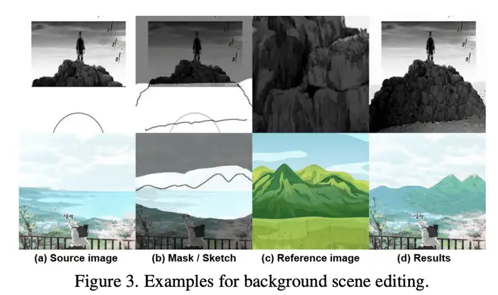
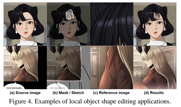
草图引导生成可用于各种情况，例如操纵对象的形状和改变姿势。当生成对象的特定部分时，获得合适的参考图像并非易事，因为很难收集带有遮蔽部分的谐波图像。在实践中，我们发现 交替使用初始图像的某一部分 是获取 参考图像 的合理方法。

3）数据集：Danbooru

文章使用了 Danbooru2021 数据集，但是由于原始数据集的体积庞大，我们选择使用其 子集 来减少过多的训练时间。The training and testing datasets comprise 55,104 and 13,775 image-sketch pairs, respectively.

1.3、实验

We employed a recently released edge detection method to extract the edges, subsequently binarizing the extracted edges.

我们采用 边缘检测方法 来提取边缘，随后对提取的边缘进行二值化

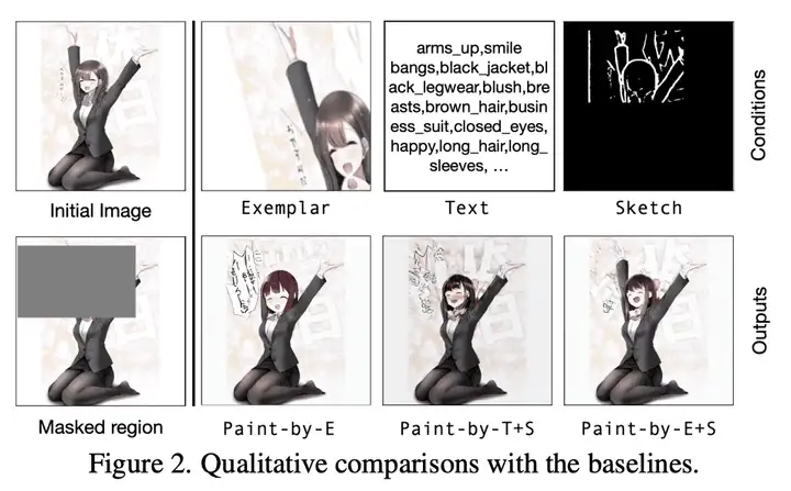
文章提供了两个 baselines：

• Paint-by-T+S：使用 Text-Sketch Pair 作为控制条件

• Paint-by-E(xample)：使用 Example Image 作为控制条件

而文章提到的方法则用 Paint-by-E+S 表示，使用 Example-Sketch Pair 作为控制条件。

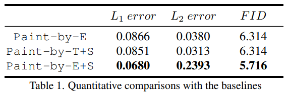
For quantitative comparison, we use the averages of L1 and L2 errors between the initial and reconstructed images. We utilize Frechet inception distance (FID) to evaluate the visual quality of the generated images.

为了进行定量比较，我们使用初始图像和重建图像之间的 L1 和 L2 误差的平均值。我们利用 FID 距离来评估生成图像的视觉质量。结果如下图所示：

下面是几个实际的例子，如下所示：

2、Long-term Forecasting with TiDE: Time-series Dense Encoder

文艺复兴：MLP 在时序预测上的应用

基于 TiDE 的长期预测：时间序列密集编码器

《Long-term Forecasting with TiDE: Time-series Dense Encoder》

• URL：https://arxiv.org/abs/2304.08424

• Official Code：未开源

• 单位：Google Research、Google Cloud

• 动机：之前的研究表明，在 长期时间序列预测（long-term time-series forecasting） 中，简单的线性模型 可以胜过几种基于 Transformer 的方法。为了解决这个问题，提出一个新的模型 TiDE（Time-series Dense Encoder），旨在解决长期时间序列预测中的协变量和非线性依赖关系，同时保留线性模型的简单和速度特点。

• 方法：TiDE 是一种 基于多层感知器的编-解码模型（Multi-layer Perceptron (MLP) based encoder-decoder model），用于长期时间序列预测。它将时间序列的过去和协变量进行编码，用密集的多层感知器进行解码预测未来的时间序列和协变量。

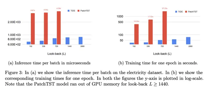
• 优势：研究表明，该模型可以 匹配或超越 之前的长期时间序列预测方法，比基于 Transformer 的最优模型 快 5-10 倍。

  • 模型推理（inference）时，快 5 倍以上

  • 模型训练（training）时，快 10 倍以上

  • Our Multi-Layer Perceptron (MLP)-based model is embarrassingly simple without any self-attention, recurrent or convolutional mechanism

    • 能够在线性时间复杂度上运行，并且在 上下文和感受野长度（context and horizon lengths） 增加的时候，仍然能够有很好的计算效率

提出一种 基于多层感知器的编-解码模型，TiDE，用于长期时间序列预测。该模型既能够处理协变量和非线性依赖关系，同时还具有线性模型的简单和快速特点。研究表明，TiDE 在流行的长期时间序列预测基准上可以匹配或超越之前的神经网络方法，比最佳 Transformer 模型快 5-10 倍。

Long-term forecasting, which is to predict several steps into the future given a long context or look-back, is one of the most fundamental problems in time series analysis, with broad applications in energy, finance, and transportation.

长期预测，即在长期背景或回顾的情况下预测未来的几个步骤，是时间序列分析中最基本的问题之一，在能源、金融和交通领域有着广泛的应用。

2.1、公式描述

主要研究长期时间多元预测（Long-term Multivariate Forecasting）这一问题，

• 数据集中的每个样本包含 \(N\) 个时间序列

• 第 \(i\) 个时间序列的回顾（look-back, history）将由 \(y^{(i)}_{1:L}\) 表示，而 horizon（要预测的时间范围，步数 \(H\)） 由 \(y^{(i)}_{L+1:L+H}\) 表示

The task of the forecaster is to predict the horizon time-points given access to the look-back.

In many forecasting scenarios, there might be dynamic and static covariates（协变量） that are known in advance.

• \(x^{(i)}_t\in R^r\) 表示第 \(i\) 个时间序列在时间 \(t\) 的 \(r\) 维动态协变量

  • 例如，它们可以是全局协变量（所有时间序列通用），例如星期几、假期等，或者特定于时间序列，例如需求预测用例中特定日期特定产品的折扣

• \(\alpha^{(i)}\) 表示第 \(i\) 个时间序列的静态属性

  • 例如，在零售需求预测中不随时间变化的产品特征

在许多应用中，这些协变量对于准确预测至关重要，一个好的模型架构需要很好地对他们进行处理。

预测器（forecaster）可以看成是一个函数，它将历史序列信息 \(y^{(i)}_{1:L}\)、动态协变量 \(x^{(i)}_{1:L+H}\) 和静态属性 \(\alpha^{(i)}\) 映射到对未来的准确预测，即：

使用 MSE 作为损失函数，如下所示：

2.2、模型结构

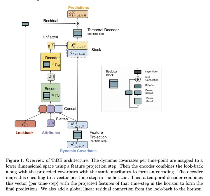
In our model we add non-linearities in the form of MLPs in a manner that can handle past data and covariates.

It encodes the past of a time-series along with covariates using dense MLP’s and then decodes the encoded time-series along with future covariates.

TiDE 以 通道独立（Channel Independent） 的方式处理 \(N\) 个时间序列，即将 \((y^{(i)}_{1:L}, x^{(i)}_{1:L}, \alpha^{(i)})\) 映射到第 \(i\) 个时间序列的 \(y^{(i)}_{L+1:L+H}\) 预测。

我们模型中的一个关键组成部分是下图右侧的 MLP 残差块。

2.3、实验结果

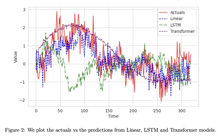
TiDE 与其他方法（LSTM、Transformers）的结果对比如下图所示，其中 actuals 表示实际的结构，即 Ground Truth。

TiDE 在时间上的高效率如下图所示：

参考

• 知乎：爱可可AI前沿推介(4.24)